
APPARATUS REQUIRED
i) Simple pendulum
ii) Stop watch
iii) Meter scale
iv) Clamp and thread
THEORY
The principle of Least Squares:
least-square is one of the most commonly used methods in numerical computation. Essentially it is a technique for solving a set of equations where there are more equations than unknowns ie. an overdetermined set of equations. This set of notes shows the origins of a particular form of the algorithm, batch linear least-squares.
The most important application is in data fitting. The best fit in the least squares sense minimizes the sum of squared residuals, a residual being the difference between an observation value and the fitted value provided by a model. When the problem has substantial uncertainties
In the independent variable, Then simple regression and least square methods leave problems: in such cases, the methodology required for fitting errors in variable models may be considered instead of that for least squares.
Least squares depending problem fall into two categories,
Linear or ordinary least squares and non-linear least squares depending on whether or not the residuals are linear are all unknown. This problem occurs in statistical regression analysis; it has a closed-form solution. A closed form solution is any formula that can be evaluated in a finite number of standard operations. The non-linear problem has no closed form solution and is usually solved by iterative refinement at which iteration is approximated by a linear one, and thus the core calculation is similar in both cases.
A residual is defined as the difference between the actual value of the dependent variable and the value predicted by the model.
γi = yi – f(xi, β)
An example of a model is that of the straight line in two dimensions. Denoting the intercept as βo and the slope as β1 the model function is given by
f(x, β) = βo + β1x
let, the equation of straight line y = a+bx – – – – – – (i)
which is fitted to given points (x1y1) (x2 y2) (x3 y3)- – – – – – – – (xn yn)
let R, be the theoretical value for x1 than, E1 = y1-R1 = y1– (d+ bx1)
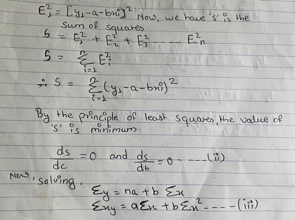
On solving equation (iii) we get the value of ‘a’ and ‘b’ and putting this value in equation (i) we get the value of equation in line of best fit.
OBSERVATION
Diameter of ball(d) = M.SR + C.SR x L.C.
= 18+50× 0.01 =18.50m
r=d/2 = 18.50/2 = 9.25cm = 0.925m
| Time for 20 Oscillation | Time forPer oscillation | Effectivelength(l) | g(ms2)4𝝅2l/T2 | Mean(g) | T2 |
| 17 | 17/20 =0.85 | 20 | 195.11 | 0.72 | |
| 25 | 25/20 =1.25 | 40 | 1011.24 | 1.56 | |
| 31 | 31/20 = 1.55 | 60 | 985.96 | 1021.95 | 2.40 |
| 35 | 35/20 = 1.75 | 80 | 1031.07 | 3.06 | |
| 40 | 40/20 = 2 | 100 | 985.96 | 4 |
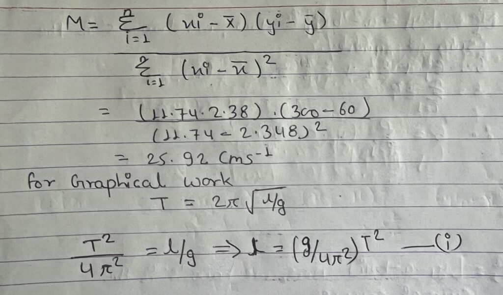
Slope of (m) =g/4𝝅2 = 1021.95/ 4×(3.14)2 = 25.92 cms-2
| Time for 20 Oscillation | Time for 1 Oscillation | T2 | Xi X1+X2+- – | x̄ | Effective length(l) | Yi Y1+y2+- – | Ȳ |
| 17 | 0.05 | 0.75 | 20 | ||||
| 25 | 1.25 | 1.56 | 11.74 | 2.348 | 40 | ||
| 31 | 1.55 | 2.40 | 60 | 300 | 60 | ||
| 35 | 1.75 | 3.06 | 80 | ||||
| 40 | 2 | 4 | 100 |
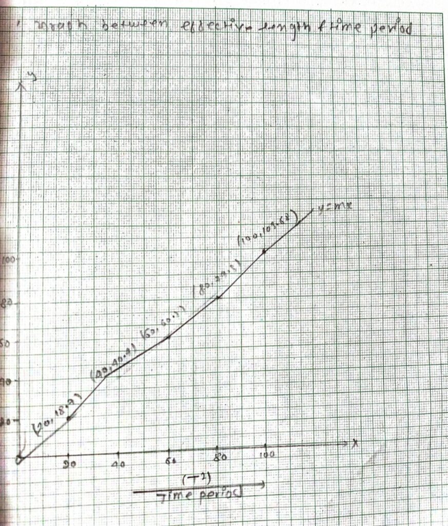
which is compared with equation of straight line y= mx
If l= 20 then l= 25.92 × 0.72 = 18.7
l= 40 then l= 25.92 × 1.56 = 40.4
l= 60 then l= 25.92 × 2.4 = 62.2
l= 80 then l= 25.92 × 3.06 = 79.31
l= 100 then l= 25.92 × 4 = 103.68
RESULT:
Thus the slope m= 25.92 and acceleration due to gravity (g) = 10.21 m/sec2
PERCENTAGE ERROR
Observed value of (o)g= 10.21 m/s²
standard value of (s)g = 9.8 m/s²
percentage errors=| 9.8-10.21/9.8 ×100%|
= 4.32
CONCLUSION:
Hence, the acceleration due to gravity can be determined by using a simple pendulum.